Hidden Markov Model Parameter Estimation: Using the EM Algorithm for Sequence Modelling

Introduction

Many real-world datasets arrive as sequences rather than independent rows. Examples include user clickstreams, machine sensor readings over time, speech signals, ECG traces, and transaction histories. In these settings, the current observation often depends on an underlying “state” that we cannot directly see—such as user intent, machine health, or phoneme category. Hidden Markov Models (HMMs) are a classic way to represent this idea: a sequence of hidden states generates a sequence of observed signals. The practical challenge is estimation—how do we learn the model parameters when the states are hidden? This is where the Expectation-Maximisation (EM) framework becomes essential. If you encounter sequence modelling in a data science course, HMM parameter estimation is a structured example of learning with latent variables.

1) Hidden Markov Models in Simple Terms

An HMM assumes two layers:

• Hidden states Z1,Z2,…,ZTZ_1, Z_2, \dots, Z_TZ1​,Z2​,…,ZT​: discrete states such as “high engagement” vs “low engagement”, or “healthy” vs “faulty”.
  
• Observed variables X1,X2,…,XTX_1, X_2, \dots, X_TX1​,X2​,…,XT​: the data we actually measure, such as clicks per minute or sensor values.
  

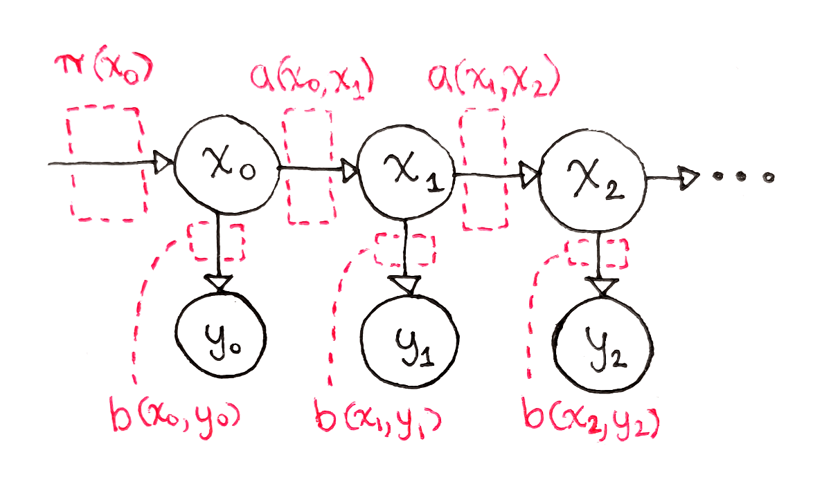
An HMM is defined by three parameter sets:

1. Initial state distribution πi=P(Z1=i)\pi_i = P(Z_1 = i)πi​=P(Z1​=i)
   
2. Transition probabilities aij=P(Zt+1=j∣Zt=i)a_{ij} = P(Z_{t+1}=j \mid Z_t=i)aij​=P(Zt+1​=j∣Zt​=i)
   
3. Emission probabilities bj(x)=P(Xt=x∣Zt=j)b_j(x) = P(X_t=x \mid Z_t=j)bj​(x)=P(Xt​=x∣Zt​=j) (discrete) or a probability density (continuous, e.g., Gaussian)
   

Given these, an HMM can generate sequences. In practice, we reverse the problem: we observe X1…XTX_1\ldots X_TX1​…XT​ and want to estimate π\piπ, AAA, and emission parameters.

2) Why Parameter Estimation Is Hard When States Are Hidden

If the state sequence were known, estimation would be straightforward: count transitions to estimate aija_{ij}aij​, count emissions to estimate bjb_jbj​, and count starting states to estimate π\piπ. But we do not observe ZtZ_tZt​. We only see XtX_tXt​, and many different hidden-state sequences can plausibly explain the same observed sequence.

This missing-information problem is exactly what EM is designed for. EM alternates between estimating the hidden variables given current parameters and updating parameters given those estimated hidden variables. In the HMM context, this is commonly called the Baum–Welch algorithm.

3) The EM Algorithm for HMMs: E-step and M-step

EM aims to maximise the likelihood P(X1:T∣θ)P(X_{1:T} \mid \theta)P(X1:T​∣θ), where θ\thetaθ represents all HMM parameters.

E-step: Compute expected hidden-state behaviour

We compute “soft” assignments—probabilities of being in each state at each time, and probabilities of transitions between states at successive times.

Key quantities are:

• State posterior
  γt(i)=P(Zt=i∣X1:T,θ)\gamma_t(i) = P(Z_t=i \mid X_{1:T}, \theta)γt​(i)=P(Zt​=i∣X1:T​,θ)
  This tells us how likely the model believes state iii was at time ttt.
  
• Transition posterior
  ξt(i,j)=P(Zt=i,Zt+1=j∣X1:T,θ)\xi_t(i,j) = P(Z_t=i, Z_{t+1}=j \mid X_{1:T}, \theta)ξt​(i,j)=P(Zt​=i,Zt+1​=j∣X1:T​,θ)
  This tells us how likely it is that the model transitioned from iii to jjj at time ttt.
  

To compute these efficiently, we use the forward–backward algorithm:

• Forward pass computes probabilities of partial observations up to time ttt given a state at ttt.
  
• Backward pass computes probabilities of future observations from time t+1t+1t+1 onward given a state at ttt.
  

This dynamic programming approach avoids enumerating all possible state sequences, which would be exponentially large.

M-step: Update parameters using expected counts

Once we have expected state occupancies and transitions, we update parameters like we would if we had counts—except now they are fractional (“expected”).

• Initial distribution:
  πi←γ1(i)\pi_i \leftarrow \gamma_1(i)πi​←γ1​(i)
• Transition probabilities:
  aij←∑t=1T−1ξt(i,j)∑t=1T−1γt(i)a_{ij} \leftarrow \frac{\sum_{t=1}^{T-1}\xi_t(i,j)}{\sum_{t=1}^{T-1}\gamma_t(i)}aij​←∑t=1T−1​γt​(i)∑t=1T−1​ξt​(i,j)​
  Numerator: expected transitions i→ji \to ji→j. Denominator: expected times in state iii.
  
• Emission parameters:
  For discrete emissions, emissions become expected frequency counts per state.
  For Gaussian emissions, you update means and variances using weighted averages where weights are γt(i)\gamma_t(i)γt​(i).
  

EM repeats E-step and M-step until the likelihood stops improving meaningfully or a maximum number of iterations is reached. In a data science course in Mumbai, learners often encounter EM first in Gaussian Mixture Models; HMMs are a natural extension where the latent structure is sequential.

4) Practical Considerations: Stability, Initialization, and Evaluation

Even though EM is conceptually clean, real usage requires care.

Initialization matters
EM can converge to local optima. Common strategies include:

• Random initial parameters with multiple restarts
  
• Using k-means on observations to initialise emissions
  
• Setting transitions with a preference for “staying” in the same state if you expect persistence
  

Numerical stability
Forward–backward involves multiplying many probabilities, which can underflow. In practice:

• Use log-space computations, or
  
• Apply scaling at each time step (common in production implementations)
  

Model selection
Choosing the number of hidden states is not automatic. You can:

• Compare log-likelihood on validation data
  
• Use AIC/BIC as approximate penalties for complexity
  
• Prefer interpretability if states correspond to business-relevant modes
  

Check whether the model is useful
Beyond likelihood, ask whether:

• Predicted state sequences align with known events (faults, promotions, outages)
  
• State transition patterns make domain sense
  
• Features derived from state posteriors improve downstream tasks (classification, alerting)
  

These evaluation habits are core in any data science course in Mumbai because they prevent “successful training” from being mistaken for “useful modelling.”

Conclusion

Hidden Markov Models provide a disciplined way to model sequences driven by unobserved states. Parameter estimation becomes challenging because those states are hidden, but the Expectation-Maximisation approach—implemented as the Baum–Welch algorithm—solves this by alternating between soft state inference (E-step via forward–backward) and parameter updates using expected counts (M-step). With good initialization, numerical safeguards, and sensible validation, EM-based HMM training becomes a reliable technique for sequence modelling problems across analytics and machine learning.

Business name: ExcelR- Data Science, Data Analytics, Business Analytics Course Training Mumbai

Address: 304, 3rd Floor, Pratibha Building. Three Petrol pump, Lal Bahadur Shastri Rd, opposite Manas Tower, Pakhdi, Thane West, Thane, Maharashtra 400602

Phone: 09108238354 

Email: enquiry@excelr.com